I have always been fascinate by the workings of the human brain and how it enables us to comprehend various sounds and understand the details of colors. With each new piece of knowledge I acquire, I realize that there are numerous concepts at play in our quest for understanding.
The human brain is very complex and advanced organ, and its ability to process information and perceive details is a result of complex neural mechanisms. However, what is the fundamental concept that underlies these processes? Mathematics and wave functions emerge as key players in explaining and comprehending the mechanisms of perception and information processing within the brain. In this blog, we will solely focus on the role of Mathematics in this regard.
Now, let's delve into a fascinating realm that bridges the sophistication of the human brain with cutting-edge technology—artificial neural networks.
Neuron
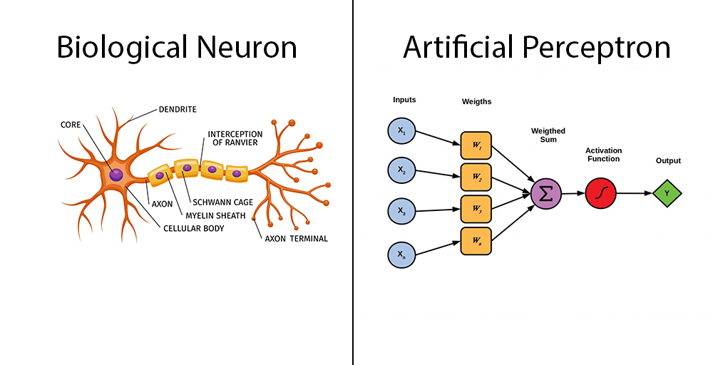
Biological Neuron
The human brain consists of a complex network of billions of interconnected neurons. Neurons play a crucial role in processing and transmitting chemical and electrical signals. Cell nucleus(core) or Soma processes the information received from dendrites. Axon is a cable that is used by neurons to send information. Synapse is the connection between an axon and other neuron dendrites. Dendrites, on the other hand, are extensions that receive information from neighboring neurons. This brief statement provides us short idea of how our neuron cell behave.
Artificial Neuron(Perceptron)
Artificial neuron, also referred to as perceptrons, serve as the fundamental building blocks of Artificial neural networks. These mathematical functions are derived from the structure of biological neurons and can be likened to basic logic gates that produce binary outputs.
Perceptron
It is the primary step to learn Machine Learning and Deep Learning technologies, which consists of a set of weights, input values or scores, and a bias. Perceptron is a building block of an Artificial Neural Network. Initially, in the mid of 19th century, Mr. Frank Rosenblatt invented the Perceptron for performing certain calculations to detect input data capabilities or business intelligence. Perceptron is a linear Machine Learning algorithm used for supervised learning for various binary classifiers. This algorithm enables neurons to learn elements and processes them one by one during preparation.

Please be patient as I provide a detailed explanation of neural networks. We will thoroughly dissect each component of the neural network, and I will also provide a Python code snippet for the mathematical equations involved. Let’s begin
Input Layer(X)
The Perceptron's main element is responsible for receiving the initial data and facilitating its subsequent processing within the system. Each input node is designed to hold a specific real numerical value.
Weight(W)
The weight parameter signifies the magnitude of the link between units. It is a crucial parameter within the Perceptron components. The weight is directly correlated to the influence of the corresponding input neuron in determining the output. In other words, The weights in an ANN are crucial because they directly influence the signals transmitted across the network and ultimately determine the network's output. During the training phase, the ANN learns by iteratively adjusting these weights to predict the correct output for a given set of inputs. The set of weights in the network encapsulates what the network has learned from the training data, effectively encoding the knowledge necessary for making predictions or decisions.
Weighted sum
In the first step first, multiply all input values with corresponding weight values and then add them to determine the weighted sum. Mathematically, we can calculate the weighted sum as follows:
import numpy as np

inputs = np.array([-4,0,2,-5])
weights = np.array([0.1,0.5,0.7,1.2])

weightsum= np.dot(inputs,weights)


# weightsum= dot(x,w)
# 5 =  dot([0,0,2,3] , [0.1,0.5,0.7,1.2])
#-5 =  dot([-4,0,2,-5] , [0.1,0.5,0.7,1.2])
Activation Function
An activation function is a mathematical operation applied to the input of a neuron in a neural network. It determines the output of the neuron, which is then used as input for the next layer in the network. Activation functions introduce non-linearity to the network, allowing it to learn and approximate complex relationships in data. but in single perceptron we have linear decision boundaries.
In the context of a single perceptron, the step function is often used as the activation function. Is a mathematical function that produces a binary output based on whether the input exceeds a specified threshold. The output is typically 1 if the input is greater than or equal to the threshold and 0 otherwise.
For more information about activations function, please visit this given Wikipedia link. -> wiki/Activation_function or this blog -> https://www.v7labs.com/blog/neural-networks-activation-functions
def step_function(weightsum):
    if(weightsum >= 0):
        return 1
    else:
        return 0

step_function(weightsum)

# weightsum= dot(x,w)

# 5 =  dot([0,0,2,3] , [0.1,0.5,0.7,1.2])
# 1 = step_function(5)

#-5 =  dot([-4,0,2,-5]  , [0.1,0.5,0.7,1.2])
# 0 = step_function(-5)
Bias
In neural network , bias refers to a constant that is added to the summation of product of features and weights. Its purpose is to adjust the outcome and assist the models in shifting the activation function towards either the positive or negative side. However, in the case of a single perceptron with a step function, the practical significance of the bias is limited. It becomes more significant in more complex neural network architectures where non-linear activation functions are used and the network needs to learn and adapt to various patterns in the data.
However, I will make an attempt to explain this with help of code.
import numpy as np

inputs = np.array([0,0,2,3])
weights = np.array([0.1,0.5,0.7,1.2])
bias = -6

weightsum= np.dot(inputs,weights) + bias

def step_function(weightsum):
    if(weightsum >= 0):
        return 1
    else:
        return 0

step_function(weightsum)

# weightsum= dot(x,w)

#bias = -6
# -1 =  dot([0,0,2,3] , [0.1,0.5,0.7,1.2]) + bias
# 0 = step_function(-1)

# bias = 6
# 1 =  dot([-4,0,2,-5] , [0.1,0.5,0.7,1.2]) + bias
# 1 = step_function(1)
This showcases how the bias term influences the decision boundary of the perceptron. Adjusting the bias allows the perceptron to shift its decision threshold, influencing whether it activates or not based on the input features.
Limitations of single perceptron
- Binary Outputs
- Inability to Learn XOR Function
- Sensitivity to Input Changes
- Not Suitable for Nonlinear Problems
- Difficulty in Training
- Single-Layer Limitation
The development of multilayer perceptrons (MLPs) was a direct response to the limitations mentioned above. These MLPs were designed specifically to address and overcome these challenges. MLP also know as Neural Network.
Neural Network
A neural network is like a team of interconnected perceptrons (basic computing units) that imitates, in a simplified way, how the human brain works. Each perceptron is connected to others, and during learning, these connections get adjusted. While it's inspired by the brain,It's a simpler model created for specific tasks, not as complex as the real thing.
Multi-Layer Perceptron
A Multi-Layer Perceptron (MLP) is a type of artificial neural network that consists of multiple layers of nodes, or neurons(Perceptrons).

Note: Forward propagation and backward propagation are terms commonly used in the context of artificial neural networks, which are a key component of ML/DL models. These processes are fundamental to training neural networks.
Forward propagation

Forward propagation, also known as forward pass or inference, is the process in which input data is passed through a neural network to generate predictions or outputs. It involves the sequential computation of the network's activations from the input layer to the output layer. The key steps in forward propagation are as follows:
- Input Layer: This layer consists of nodes that represent the input features of the model. Each node corresponds to a feature of the input data.
- Hidden Layers: Between the input and output layers, there can be one or more hidden layers. Each hidden layer contains nodes that perform computations on the input data. These layers are responsible for learning patterns and representations from the input.
- Output Layer: The output layer produces the final result of the network's computation. The number of nodes in the output layer depends on the type of problem the MLP is designed to solve. For example, in a binary classification problem, there might be one node for each class.
Let's break the Forward propagation
equation to calculat forward pass We can compute this formula for every output neuron in one shot using a dot product :
module.py (base class for all layers)
# Base class
class Module:
    def __init__(self):
       pass

    def forward(self, input_features: float):
        raise NotImplementedError("Subclasses must implement my_abstract_method")

    def backpropagation(self, output_error: float, learning_rate: float):
        raise NotImplementedError("Subclasses must implement my_abstract_method")
linear.py (implement our equation)
from module import Module
import numpy as np

class Linear(Module):
    def __init__(self, input_size: int, output_size: int, bias: bool = True, w_b_range: float = 0.5):
        # Initialize weights with random values between -w_b_range and w_b_range
        self.weights = np.random.rand(input_size, output_size) - w_b_range

        # Initialize bias if bias is True, otherwise set bias to 0.0
        self.bias = np.random.rand(1, output_size) - w_b_range if bias else 0.0

    def forward(self, input_features: float):
        self.input_features = input_features
        self.out_features = np.dot(self.input_features, self.weights) + self.bias
        return self.out_features
These are activation functions i am using in this code.
- Relu
- Equation:
- Image

- Sigmoid
- Equation:
- Image

activation.py
from module import Module
import numpy as np

class ReLU(Module):
    def __init__(self):
        # Constructor, but it's empty in this case
        pass

    def forward(self, input_features):
        # Forward pass of the ReLU activation function
        # Save the input features for potential use in backward pass
        self.input_features = input_features

        # Apply ReLU activation element-wise
        self.activation = np.maximum(0, self.input_features)

        # Return the result of the activation
        return self.activation


class Sigmoid(Module):
    def __init__(self):
        # Constructor, but it's empty in this case
        pass

    def sigmoid(self, x):
        return 1 / (1 + np.exp(-x))

    def forward(self, input_features):
        # Forward pass of the sigmoid activation function
        # Save the input features for potential use in the backward pass
        self.input_features = input_features

        # Apply the sigmoid activation element-wise
        self.activation = self.sigmoid(self.input_features)

        # Return the result of the activation
        return self.activation
writing custom model like pytorch.
mlp.py
from module import Module
from linear import Linear
from activation import ReLU,Sigmoid
class MLP(Module):
    # define model elements
    def __init__(self, input_size:int, output_size:int  , h_l_dimension:int = 10):

        self.h_l_dimension = h_l_dimension
        # input to first hidden layer
        self.hidden1 = Linear(input_size, self.h_l_dimension)
        self.act1 = ReLU()
        # second hidden layer
        self.hidden2 = Linear(self.h_l_dimension, self.h_l_dimension)
        self.act2 = ReLU()
        # third hidden layer and output
        self.hidden3 = Linear(self.h_l_dimension , output_size)
        self.act3 = Sigmoid()

    # forward propagate input
    def forward(self, input_features: float ):
        # input to first hidden layer

        X = self.hidden1.forward(input_features)
        X = self.act1.forward(X)


        # second hidden layer
        X = self.hidden2.forward(X)
        X = self.act2.forward(X)

        # third hidden layer and output
        X = self.hidden3.forward(X)
        X = self.act3.forward(X)
        return X
main.py (run our model)
import numpy as np
from mlp import MLP

x_train = np.array([[[0,0]], [[0,1]], [[1,0]], [[1,1]]])
# One-hot encoding for binary classification:
# - [1, 0] represents the class label 0
# - [0, 1] represents the class label 1
y_train = np.array([[[1, 0]],   # Class 0
                   [[0, 1]],    # Class 1
                   [[0, 1]],    # Class 1
                   [[1, 0]]])   # Class 0

def predict_and_print_results( model , input_data, target_data):
    num_samples = len(input_data)

    for sample_index in range(num_samples):
        input_sample = input_data[sample_index]
        predicted_output = model.forward(input_sample)

        actual_output = 0 if target_data[sample_index][0][0] == 1 else 1

        print(f'{predicted_output[0] }')

        if predicted_output[0][0] >= 0.5:
            print(f'1st input for XOR: {input_sample[0][0]} 2nd input for XOR: {input_sample[0][1]} '
                  f'Neural Network output is 0, actual output is: {actual_output}')
        else:
            print(f'1st input for XOR: {input_sample[0][0]} 2nd input for XOR: {input_sample[0][1]} '
                  f'Neural Network output is 1, actual output is: {actual_output}')


model = MLP(input_size=2 ,output_size=2 , hiddenlayer=3 ,h_l_dimension=20)
predict_and_print_results(model , x_train, y_train )
output
[0.44724273 0.54032146]
1st input for XOR: 0 2nd input for XOR: 0 Neural Network output is 1, actual output is: 0
[0.4875954 0.54962158]
1st input for XOR: 0 2nd input for XOR: 1 Neural Network output is 1, actual output is: 1
[0.46728592 0.5354989 ]
1st input for XOR: 1 2nd input for XOR: 0 Neural Network output is 1, actual output is: 1
[0.51449871 0.55993924]
1st input for XOR: 1 2nd input for XOR: 1 Neural Network output is 0, actual output is: 0
Are we doing something wrong? Why is our output like this?
My answer is no. Till now our MLP model doesn't know how to find patterns inside the logic.
In simpler terms, the MLP lacks the ability to optimize its weight and bias values in order to produce the desired output. To overcome this limitation, we need to delve into the concept of backward propagation.
To grasp the concept of backward propagation, it is essential to familiarize ourselves with several smaller concepts beforehand. I apologize for not being able to cover all the concepts here. I recommend you to go over the concepts of Differential Calculus and the concept of Chain Rule. "Those things are really mandatory".
Loss or Cost function

A loss function, often referred to as a cost function in machine learning, is a critical element in training models. It will find errors between predicted and actual outcomes, serving as a guide for optimization during the learning process.
In my approach, I am utilizing the Mean Squared Error (MSE), which measures the average squared difference between predictions and true values. MSE is a widely used cost function in deep learning, providing a comprehensive assessment of model performance by penalizing larger errors more significantly.
Equation for Mean Squared Error
losses.py
def mse(y_true, y_pred):
    return np.mean(np.power(y_pred-y_true, 2))
Check out the website for a more in-depth explanation. https://builtin.com/machine-learning/cost-function
Gradient Descent
Gradient Descent is an iterative optimization algorithm used to minimize the error or cost function in machine learning and optimization problems. It works by adjusting parameters in the direction of steepest decrease of the function, as indicated by the negative gradient. This process is repeated until a minimum or satisfactory solution is reached. We want to change some parameter in the MLP so that the total Cost fucntion decreases.
In above equation is the weight being updated, is the learning rate controlling the step size, and is the gradient of the cost function with respect to the weight, guiding the update direction.
Check out the website for a more in-depth explanation. https://builtin.com/data-science/gradient-descent
Backward propagation

Backward propagation, also known as the backward pass, is the phase in the training of neural networks where the model learns and adjusts its weights based on the computed error. This iterative process is crucial for refining the network's performance. The discovery of backpropagation, credited to researchers like Paul Werbos in the 1974, laid the groundwork for this key training algorithm. The key steps in backward propagation are as follows:
-
Calculate Error: The first step in the backward pass involves computing the error by comparing the predicted output generated during the forward pass with the actual target values. This error is a measure of how well the model is performing on the given task.
-
Compute Gradients: The gradient of the loss with respect to each weight in the network is calculated. This is achieved using the chain rule of calculus, breaking down the overall gradient into contributions from each layer. The gradient provides information about how the loss would change with a small adjustment to each weight.
-
Update Weights: The calculated gradients are used to update the weights of the neural network. This step involves adjusting the weights in the opposite direction of the gradients, aiming to minimize the error. Optimization algorithms, such as gradient descent, are often employed for this purpose.
Sounds like Backward propagation and gradient descent are interconnected.
Backward propagation at the output layer

It appears that there are numerous activities taking place in the image above. Don't worry, we are breaking down the backpropagation process for the output layer with respect to . This involves computing the gradient of the Cost function with respect to and subsequently using gradient descent, an optimization algorithm, to update the weight in order to minimize the overall loss during training.
But here's the catch: we cannot directly perform partial differentiation of the cost function with respect to . We have to split the equation into multiple terms, applying the chain rule to handle each part separately.
In general, Most of the time we observe that the chain rule for partial differentiation of the cost function with respect to weight consists of only two terms:
- the partial differentiation of the cost function with respect to the output
- the partial differentiation of the output with respect to the weight.
So, together, the expressions can be written as:
However, we have included the activation function between the cost function and the summation of weights and input features. This means we cannot directly perform ; we have to expand it further.
- considering the partial differentiation of the cost function with respect to the activation function, denoted as .
- the partial differentiation of the activation function with respect to the output.
Here activation function is Sigmoid function.
Now, new equation written as:
Now, we calculate each term individually to derive equations that will assist us in writing Python code.
Partial differentiation of the cost function with respect to the activation function. Basically, it is the derivative of the Mean Squared Error.
losses.py
def mse_derivative(y_true, y_pred):
    return (2/y_true.size) * (y_pred - y_true)
finding derivative of sigmoid function.
If you want to know how the sigmoid function is derived step by step, make sure to check out the provided website. Derivative of Neural Activation Function
activation.py
class Sigmoid(Module):

  def sigmoid_derivative(self, x):
        # Derivative of the sigmoid activation function
        sigmoid_x = self.sigmoid(x)
        return sigmoid_x * (1 - sigmoid_x)

  #here output_error is dC/dS
  #Remember we are doing Element-wise products between sigmoid_derivative and output_error
  def backpropagation(self, output_error: float, learning_rate: float):
        return self.sigmoid_derivative(self.input_features) * output_error
Now, for the final term .
What about bais?
We can take
output_error
linear.py
class Linear(Module):
    # here output_error can be dC/dS x dS/dy or dC/dR x dR/dH depend on activation function and layer type
    def backpropagation(self, output_error, learning_rate):

        weights_error = np.dot( self.input_features.T, output_error)

        # Update weights and bias using gradient descent
        self.weights -= learning_rate * weights_error
        self.bias -= learning_rate * output_error
Backward propagation at Hidden layer

In this section, we are breaking down the backpropagation process for the hidden layer with respect to .
The biggest question will arise. how we can find (here R is ReLU activation function). And what is input from output layer?
Using the chain rule, we can expand this equation to.
With the help of this equation, we can find the input from output layer.
We have and , but we dont know what is this term for.

Now, we can find
linear.py
class Linear(Module):
    # here output_error can be dC/dS x dS/dy or dC/dR x dR/dH depend on activation function and layer type
    def backpropagation(self, output_error, learning_rate):

        #input_error is input for previous layer
        input_error = np.dot(output_error, self.weights.T)
        weights_error = np.dot( self.input_features.T, output_error)

        # Update weights and bias using gradient descent
        self.weights -= learning_rate * weights_error
        self.bias -= learning_rate * output_error
        return input_error
finding derivative of ReLU function.
activation.py
class ReLU(Module):

    def relu_derivative(self, x):
        # Subgradient of the ReLU activation function
        return np.where(x >= 0, 1, 0)

    #here output_error is dC/dR
    #Remember we are doing Element-wise products between relu_derivative and output_error
    def backpropagation(self, output_error: float, learning_rate: float):
        return self.relu_derivative(self.input_features) * output_error
Now, for the final term .
Writing every layer in reverse order.
mlp.py
class MLP(Module):
    def backpropagation(self, output_error: float, learning_rate: float):
        X = self.act3.backpropagation(output_error, learning_rate)
        X = self.hidden3.backpropagation(X, learning_rate)


        # second hidden layer
        X = self.act2.backpropagation(X, learning_rate)
        X = self.hidden2.backpropagation(X, learning_rate)


        X = self.act1.backpropagation(X , learning_rate)
        X = self.hidden1.backpropagation(X , learning_rate)
The whole process of moving information through the network (forward pass) and learning from mistakes (backward pass) makes up one round of training. We do this a bunch of times (iterations or epochs), thanks to the discovery of backpropagation. We can adjust the weights with this automated process.
Epoch
- An epoch corresponds to a single, complete cycle through the entire training dataset while the model is being trained.
- In each epoch, the model encounters and learns from every example in the training set exactly once.
- Training a model for multiple epochs allows it to see the entire dataset multiple times, refining its parameters and improving performance.
Batch Size
- Batch size refers to the number of training examples utilized in one iteration.
- In each iteration (or training step), the model processes a batch of data instead of the entire dataset.
- Batch size influences the speed of training, memory requirements, and the stochastic nature of the optimization process.
Finally, we have implemented every step to train our neural network.
main.py
   import numpy as np
   from mlp import MLP
   from losses import mse, mse_derivative

   x_train = np.array([[[0,0]], [[0,1]], [[1,0]], [[1,1]]])
   # One-hot encoding for binary classification:
   # - [1, 0] represents the class label 0
   # - [0, 1] represents the class label 1
   y_train = np.array([[[1, 0]],   # Class 0
                      [[0, 1]],    # Class 1
                      [[0, 1]],    # Class 1
                      [[1, 0]]])   # Class 0

   def predict_and_print_results( model , input_data, target_data):
       num_samples = len(input_data)

       for sample_index in range(num_samples):
           input_sample = input_data[sample_index]
           predicted_output = model.forward(input_sample)

           actual_output = 0 if target_data[sample_index][0][0] == 1 else 1

           print(f'{predicted_output[0] }')

           if predicted_output[0][0] >= 0.5:
               print(f'1st input for XOR: {input_sample[0][0]} 2nd input for XOR: {input_sample[0][1]} '
                     f'Neural Network output is 0, actual output is: {actual_output}')
           else:
               print(f'1st input for XOR: {input_sample[0][0]} 2nd input for XOR: {input_sample[0][1]} '
                     f'Neural Network output is 1, actual output is: {actual_output}')


   def train_neural_network(model, input_data, target_data, num_epochs, learning_rate):
       # Get the number of samples
       num_samples = len(input_data)

       # Training loop
       for epoch in range(num_epochs):
           total_error = 0

           for sample_index in range(num_samples):
               # Forward propagation
               input_sample = input_data[sample_index]
               predicted_output = model.forward(input_sample)

               # Compute loss
               total_error += mse(target_data[sample_index], predicted_output)

               # Backward propagation
               output_error = mse_derivative(target_data[sample_index], predicted_output)
               model.backpropagation(output_error, learning_rate)

           # Calculate the average error on all samples
           average_error = total_error / num_samples
           print(f'Epoch {epoch + 1}/{num_epochs}   Mean Squared Error: {average_error:.6f}')


   model = MLP(input_size=2 ,output_size=2 , h_l_dimension=20)
   train_neural_network(model , x_train, y_train, num_epochs=3000, learning_rate=0.1)
   predict_and_print_results(model , x_train, y_train )
output
Epoch 2996/3000 Mean Squared Error: 0.000011
Epoch 2997/3000 Mean Squared Error: 0.000011
Epoch 2998/3000 Mean Squared Error: 0.000011
Epoch 2999/3000 Mean Squared Error: 0.000011
Epoch 3000/3000 Mean Squared Error: 0.000011
[0.99599307 0.00387084]
1st input for XOR: 0 2nd input for XOR: 0 Neural Network output is 0, actual output is: 0
[0.00277158 0.99691068]
1st input for XOR: 0 2nd input for XOR: 1 Neural Network output is 1, actual output is: 1
[0.00241043 0.99837826]
1st input for XOR: 1 2nd input for XOR: 0 Neural Network output is 1, actual output is: 1
[0.99599521 0.00353148]
1st input for XOR: 1 2nd input for XOR: 1 Neural Network output is 0, actual output is: 0
Our MLP able to solve XOR problem.
Full code is available on GitHub
If you are crazy and want to solve these equations on paper here is the link for you Backpropagation Process